导入相关包
import numpy as np
import pandas as pd
导入numpy与pandas的工具包
对象创建
通过series创建
s=pd.Series([1, 3, 5, np.nan, 6, 8])
s
0    1.0
1    3.0
2    5.0
3    NaN
4    6.0
5    8.0
dtype: float64
通过dataframe创建
先创建时间索引
dates=pd.date_range('20130101',periods=6)
dates
Out[6]:
DatetimeIndex(['2013-01-01', '2013-01-02', '2013-01-03', '2013-01-04',
               '2013-01-05', '2013-01-06'],
              dtype='datetime64[ns]', freq='D')
df=pd.DataFrame(np.random.randn(6,4),index=dates,columns=list('ABCD'))
df
| A | B | C | D | |
|---|---|---|---|---|
| 2013-01-01 | 1.586798 | -1.817532 | -1.174984 | 0.399674 |
| 2013-01-02 | -0.272984 | -0.381050 | 1.547809 | 0.241587 |
| 2013-01-03 | 0.538715 | 0.214234 | 0.344610 | 0.423814 |
| 2013-01-04 | 1.950835 | -0.896320 | -1.581542 | 1.538713 |
| 2013-01-05 | 0.408649 | 0.701028 | -1.964295 | -0.001575 |
| 2013-01-06 | -1.183035 | -0.773940 | -1.387948 | -0.961777 |
dataframe通过dict创建
df2=pd.DataFrame({'A': 1.,
                  'B': pd.Timestamp('20130102'),
                  'C': pd.Series(1, index=list(range(4)), dtype='float32'),
                  'D': np.array([3] * 4, dtype='int32'),
                  'E': pd.Categorical(["test", "train", "test", "train"]), 'F': 'foo'})
df2
| A | B | C | D | E | F | |
|---|---|---|---|---|---|---|
| 0 | 1.0 | 2013-01-02 | 1.0 | 3 | test | foo |
| 1 | 1.0 | 2013-01-02 | 1.0 | 3 | train | foo |
| 2 | 1.0 | 2013-01-02 | 1.0 | 3 | test | foo |
| 3 | 1.0 | 2013-01-02 | 1.0 | 3 | train | foo |
每个列具有不同的dtypes
df2.dtypes
A           float64
B    datetime64[ns]
C           float32
D             int32
E          category
F            object
dtype: object
查看数据
查看数据的顶行和底行:
df.head(3)
Out:
| A | B | C | D | |
|---|---|---|---|---|
| 2013-01-01 | 1.586798 | -1.817532 | -1.174984 | 0.399674 |
| 2013-01-02 | -0.272984 | -0.381050 | 1.547809 | 0.241587 |
| 2013-01-03 | 0.538715 | 0.214234 | 0.344610 | 0.423814 |
df.tail(3)
Out:
| A | B | C | D | |
|---|---|---|---|---|
| 2013-01-04 | 1.950835 | -0.896320 | -1.581542 | 1.538713 |
| 2013-01-05 | 0.408649 | 0.701028 | -1.964295 | -0.001575 |
| 2013-01-06 | -1.183035 | -0.773940 | -1.387948 | -0.961777 |
显示索引与列
df.index
Out:
DatetimeIndex(['2013-01-01', '2013-01-02', '2013-01-03', '2013-01-04',
               '2013-01-05', '2013-01-06'],
              dtype='datetime64[ns]', freq='D')
df.columns
Out:
Index(['A', 'B', 'C', 'D'], dtype='object')
显示数据快速统计摘要
df.describe()
Out[21]:
| A | B | C | D | |
|---|---|---|---|---|
| count | 6.000000 | 6.000000 | 6.000000 | 6.000000 |
| mean | 0.504830 | -0.492263 | -0.702725 | 0.273406 |
| std | 1.159816 | 0.887062 | 1.357811 | 0.805217 |
| min | -1.183035 | -1.817532 | -1.964295 | -0.961777 |
| 25% | -0.102576 | -0.865725 | -1.533143 | 0.059215 |
| 50% | 0.473682 | -0.577495 | -1.281466 | 0.320630 |
| 75% | 1.324777 | 0.065413 | -0.035289 | 0.417779 |
| max | 1.950835 | 0.701028 | 1.547809 | 1.538713 |
转置数据(行列转换)
df.T
| 2013-01-01 00:00:00 | 2013-01-02 00:00:00 | 2013-01-03 00:00:00 | 2013-01-04 00:00:00 | 2013-01-05 00:00:00 | 2013-01-06 00:00:00 | |
|---|---|---|---|---|---|---|
| A | 1.586798 | -0.272984 | 0.538715 | 1.950835 | 0.408649 | -1.183035 |
| B | -1.817532 | -0.381050 | 0.214234 | -0.896320 | 0.701028 | -0.773940 |
| C | -1.174984 | 1.547809 | 0.344610 | -1.581542 | -1.964295 | -1.387948 |
| D | 0.399674 | 0.241587 | 0.423814 | 1.538713 | -0.001575 | -0.961777 |
按索引排序
df.sort_index(axis=1,ascending=False)
| D | C | B | A | |
|---|---|---|---|---|
| 2013-01-01 | -1.415859 | 0.357454 | -0.219970 | -0.464958 |
| 2013-01-02 | -1.363227 | -0.504517 | -0.848231 | -0.349901 |
| 2013-01-03 | 0.177325 | -1.269695 | 1.289740 | 0.298251 |
| 2013-01-04 | -0.875406 | -0.099774 | 1.526283 | 0.236369 |
| 2013-01-05 | -0.715345 | 0.842110 | -1.966019 | -0.703749 |
| 2013-01-06 | 1.972990 | -1.115897 | 0.440815 | 1.061018 |
按值排序
df.sort_values(by='B')
| A | B | C | D | |
|---|---|---|---|---|
| 2013-01-05 | -0.703749 | -1.966019 | 0.842110 | -0.715345 |
| 2013-01-02 | -0.349901 | -0.848231 | -0.504517 | -1.363227 |
| 2013-01-01 | -0.464958 | -0.219970 | 0.357454 | -1.415859 |
| 2013-01-06 | 1.061018 | 0.440815 | -1.115897 | 1.972990 |
| 2013-01-03 | 0.298251 | 1.289740 | -1.269695 | 0.177325 |
| 2013-01-04 | 0.236369 | 1.526283 | -0.099774 | -0.875406 |
数据访问
获取
选择一列,获取到一个Series
df['A']
2013-01-01   -0.464958
2013-01-02   -0.349901
2013-01-03    0.298251
2013-01-04    0.236369
2013-01-05   -0.703749
2013-01-06    1.061018
Freq: D, Name: A, dtype: float64
通过[]获取行
df[0:3]
| A | B | C | D | |
|---|---|---|---|---|
| 2013-01-01 | -0.464958 | -0.219970 | 0.357454 | -1.415859 |
| 2013-01-02 | -0.349901 | -0.848231 | -0.504517 | -1.363227 |
| 2013-01-03 | 0.298251 | 1.289740 | -1.269695 | 0.177325 |
df['20130102':'20130104']
| A | B | C | D | |
|---|---|---|---|---|
| 2013-01-02 | -0.349901 | -0.848231 | -0.504517 | -1.363227 |
| 2013-01-03 | 0.298251 | 1.289740 | -1.269695 | 0.177325 |
| 2013-01-04 | 0.236369 | 1.526283 | -0.099774 | -0.875406 |
通过标签选择(loc)
选择第一个日期的数据
df.loc[dates[0]]
A   -0.464958
B   -0.219970
C    0.357454
D   -1.415859
Name: 2013-01-01 00:00:00, dtype: float64
通过标签选择多个维度:
df.loc[:,['A','B']]
| A | B | |
|---|---|---|
| 2013-01-01 | -0.464958 | -0.219970 |
| 2013-01-02 | -0.349901 | -0.848231 |
| 2013-01-03 | 0.298251 | 1.289740 |
| 2013-01-04 | 0.236369 | 1.526283 |
| 2013-01-05 | -0.703749 | -1.966019 |
| 2013-01-06 | 1.061018 | 0.440815 |
显示数据的切片,包含两个端点数据
df.loc['20130102':'20130104', ['A', 'B']]
| A | B | |
|---|---|---|
| 2013-01-02 | -0.349901 | -0.848231 |
| 2013-01-03 | 0.298251 | 1.289740 |
| 2013-01-04 | 0.236369 | 1.526283 |
缩小返回对象的大小
df.loc['20130102', ['A', 'B']]
A   -0.349901
B   -0.848231
Name: 2013-01-02 00:00:00, dtype: float64
获取标量值
df.loc[dates[0],'A']
-0.4649577235434288
快速访问标量
df.at[dates[0], 'A']
-0.4649577235434288
通过位置选择(iloc)
通过传递的整数位置选择
df.iloc[3]
A    0.236369
B    1.526283
C   -0.099774
D   -0.875406
Name: 2013-01-04 00:00:00, dtype: float64
通过整数进行切片,类似于python、numpy
df.iloc[3:5,0:2]
| A | B | |
|---|---|---|
| 2013-01-04 | 0.236369 | 1.526283 |
| 2013-01-05 | -0.703749 | -1.966019 |
通过整数位置进行列举,类似于numpy、python
df.iloc[[1,2,4],[0,2]]
| A | C | |
|---|---|---|
| 2013-01-02 | -0.349901 | -0.504517 |
| 2013-01-03 | 0.298251 | -1.269695 |
| 2013-01-05 | -0.703749 | 0.842110 |
对行进行切片
df.iloc[1:3,:]
| A | B | C | D | |
|---|---|---|---|---|
| 2013-01-02 | -0.349901 | -0.848231 | -0.504517 | -1.363227 |
| 2013-01-03 | 0.298251 | 1.289740 | -1.269695 | 0.177325 |
对列进行切片
df.iloc[:,1:3]
| B | C | |
|---|---|---|
| 2013-01-01 | -0.219970 | 0.357454 |
| 2013-01-02 | -0.848231 | -0.504517 |
| 2013-01-03 | 1.289740 | -1.269695 |
| 2013-01-04 | 1.526283 | -0.099774 |
| 2013-01-05 | -1.966019 | 0.842110 |
| 2013-01-06 | 0.440815 | -1.115897 |
快速访问标量:
df.iat[1,1]
-0.8482314332197409
布尔值索引
通过判断单列的值选择数据
df[df.A>0]
| A | B | C | D | |
|---|---|---|---|---|
| 2013-01-03 | 0.298251 | 1.289740 | -1.269695 | 0.177325 |
| 2013-01-04 | 0.236369 | 1.526283 | -0.099774 | -0.875406 |
| 2013-01-06 | 1.061018 | 0.440815 | -1.115897 | 1.972990 |
从满足布尔条件的dataframe中选择值
df[df>0]
| A | B | C | D | |
|---|---|---|---|---|
| 2013-01-01 | NaN | NaN | 0.357454 | NaN |
| 2013-01-02 | NaN | NaN | NaN | NaN |
| 2013-01-03 | 0.298251 | 1.289740 | NaN | 0.177325 |
| 2013-01-04 | 0.236369 | 1.526283 | NaN | NaN |
| 2013-01-05 | NaN | NaN | 0.842110 | NaN |
| 2013-01-06 | 1.061018 | 0.440815 | NaN | 1.972990 |
使用isin()方法筛选
df2=df.copy()
df2['E']=['one', 'one', 'two', 'three', 'four', 'three']
df2
| A | B | C | D | E | |
|---|---|---|---|---|---|
| 2013-01-01 | -0.464958 | -0.219970 | 0.357454 | -1.415859 | one |
| 2013-01-02 | -0.349901 | -0.848231 | -0.504517 | -1.363227 | one |
| 2013-01-03 | 0.298251 | 1.289740 | -1.269695 | 0.177325 | two |
| 2013-01-04 | 0.236369 | 1.526283 | -0.099774 | -0.875406 | three |
| 2013-01-05 | -0.703749 | -1.966019 | 0.842110 | -0.715345 | four |
| 2013-01-06 | 1.061018 | 0.440815 | -1.115897 | 1.972990 | three |
df2[df2['E'].isin(['two','four'])]
| A | B | C | D | E | |
|---|---|---|---|---|---|
| 2013-01-03 | 0.298251 | 1.289740 | -1.269695 | 0.177325 | two |
| 2013-01-05 | -0.703749 | -1.966019 | 0.842110 | -0.715345 | four |
设置
设置新列自动根据索引更新数据
sl=pd.Series([1,2,3,4,5,6],index=pd.date_range('20130102',periods=6))
sl
2013-01-02    1
2013-01-03    2
2013-01-04    3
2013-01-05    4
2013-01-06    5
2013-01-07    6
Freq: D, dtype: int64
df2=df.copy()
df2[df2>0]=-df2
df2
| A | B | C | D | F | |
|---|---|---|---|---|---|
| 2013-01-01 | 0.000000 | 0.000000 | -0.357454 | -5 | NaN |
| 2013-01-02 | -0.349901 | -0.848231 | -0.504517 | -5 | -1.0 |
| 2013-01-03 | -0.298251 | -1.289740 | -1.269695 | -5 | -2.0 |
| 2013-01-04 | -0.236369 | -1.526283 | -0.099774 | -5 | -3.0 |
| 2013-01-05 | -0.703749 | -1.966019 | -0.842110 | -5 | -4.0 |
| 2013-01-06 | -1.061018 | -0.440815 | -1.115897 | -5 | -5.0 |
缺失数据
pandas使用np.nan表示缺失数据,默认不加入训练。
reindex允许更改、添加、删除指令轴上的索引,返回数据的副本
df1=df.reindex(index=dates[0:4],columns=list(df.columns)+['E'])
df1.loc[dates[0]:dates[1], 'E'] = 1
df1
| A | B | C | D | F | E | |
|---|---|---|---|---|---|---|
| 2013-01-01 | 0.000000 | 0.000000 | 0.357454 | 5 | NaN | 1.0 |
| 2013-01-02 | -0.349901 | -0.848231 | -0.504517 | 5 | 1.0 | 1.0 |
| 2013-01-03 | 0.298251 | 1.289740 | -1.269695 | 5 | 2.0 | NaN |
| 2013-01-04 | 0.236369 | 1.526283 | -0.099774 | 5 | 3.0 | NaN |
丢弃存在缺失数据的行
df1.dropna(how='any')
| A | B | C | D | F | E | |
|---|---|---|---|---|---|---|
| 2013-01-02 | -0.349901 | -0.848231 | -0.504517 | 5 | 1.0 | 1.0 |
填充缺失值
df1.fillna(value=5)
| A | B | C | D | F | E | |
|---|---|---|---|---|---|---|
| 2013-01-01 | 0.000000 | 0.000000 | 0.357454 | 5 | 5.0 | 1.0 |
| 2013-01-02 | -0.349901 | -0.848231 | -0.504517 | 5 | 1.0 | 1.0 |
| 2013-01-03 | 0.298251 | 1.289740 | -1.269695 | 5 | 2.0 | 5.0 |
| 2013-01-04 | 0.236369 | 1.526283 | -0.099774 | 5 | 3.0 | 5.0 |
获取是否为nan值的boolean掩码
pd.isna(df1)
| A | B | C | D | F | E | |
|---|---|---|---|---|---|---|
| 2013-01-01 | False | False | False | False | True | False |
| 2013-01-02 | False | False | False | False | False | False |
| 2013-01-03 | False | False | False | False | False | True |
| 2013-01-04 | False | False | False | False | False | True |
运算
运算通常不包含缺失值
统计数据
进行描述性统计
df.mean()
A    0.090331
B    0.073765
C   -0.298387
D    5.000000
F    3.000000
dtype: float64
在其他轴上的运算
df.mean(1)
2013-01-01    1.339364
2013-01-02    0.859470
2013-01-03    1.463659
2013-01-04    1.932575
2013-01-05    1.434468
2013-01-06    2.077187
Freq: D, dtype: float64
在不同维度的对象上进行运算,pandas自动进行广播
s=pd.Series([1, 3, 5, np.nan, 6, 8],index=dates).shift(2)
s
2013-01-01    NaN
2013-01-02    NaN
2013-01-03    1.0
2013-01-04    3.0
2013-01-05    5.0
2013-01-06    NaN
Freq: D, dtype: float64
df.sub(s,axis='index')
| A | B | C | D | F | |
|---|---|---|---|---|---|
| 2013-01-01 | NaN | NaN | NaN | NaN | NaN |
| 2013-01-02 | NaN | NaN | NaN | NaN | NaN |
| 2013-01-03 | -0.701749 | 0.289740 | -2.269695 | 4.0 | 1.0 |
| 2013-01-04 | -2.763631 | -1.473717 | -3.099774 | 2.0 | 0.0 |
| 2013-01-05 | -5.703749 | -6.966019 | -4.157890 | 0.0 | -1.0 |
| 2013-01-06 | NaN | NaN | NaN | NaN | NaN |
对数据运用函数
df.apply(np.cumsum)
| A | B | C | D | F | |
|---|---|---|---|---|---|
| 2013-01-01 | 0.000000 | 0.000000 | 0.357454 | 5 | NaN |
| 2013-01-02 | -0.349901 | -0.848231 | -0.147063 | 10 | 1.0 |
| 2013-01-03 | -0.051650 | 0.441509 | -1.416758 | 15 | 3.0 |
| 2013-01-04 | 0.184719 | 1.967791 | -1.516532 | 20 | 6.0 |
| 2013-01-05 | -0.519030 | 0.001772 | -0.674423 | 25 | 10.0 |
| 2013-01-06 | 0.541987 | 0.442587 | -1.790320 | 30 | 15.0 |
df.apply(lambda x:x.max()-x.min())
A    1.764767
B    3.492301
C    2.111804
D    0.000000
F    4.000000
dtype: float64
柱状图
s=pd.Series(np.random.randint(0,7,size=10))
s
0    2
1    6
2    3
3    1
4    6
5    4
6    4
7    6
8    6
9    6
dtype: int64
字符串的方法
Series在str属性中配备了一组字符串处理方法,可以方便的对数组的每个元素进行操作,并且模式匹配通常使用正则表达式
s=pd.Series(['A', 'B', 'C', 'Aaba', 'Baca', np.nan, 'CABA', 'dog', 'cat'])
s.str.lower()
0       a
1       b
2       c
3    aaba
4    baca
5     NaN
6    caba
7     dog
8     cat
dtype: object
合并
连接
pandas提供了各种工具,可以方便的将Series、DataFrame和Panel对象组合在一起,并在连接、合并类型操作的情况下,为索引和关系代数功能提供各种集合逻辑
df=pd.DataFrame(np.random.randn(10,4))
df
| 0 | 1 | 2 | 3 | |
|---|---|---|---|---|
| 0 | -2.115351 | -0.715676 | 0.307033 | 1.042703 |
| 1 | 0.957212 | -0.310875 | 0.978699 | 0.597034 |
| 2 | 0.034715 | 1.315929 | -2.278538 | -1.652614 |
| 3 | -0.729501 | 0.650241 | 0.783674 | -2.251146 |
| 4 | 0.440467 | 0.510737 | -0.208779 | -0.693988 |
| 5 | -0.017431 | -0.677659 | 0.792783 | 1.583612 |
| 6 | -1.180695 | 0.824008 | -0.687270 | 0.705201 |
| 7 | 1.579882 | -0.300540 | 0.210331 | 0.757258 |
| 8 | -1.758054 | 0.096074 | -1.010636 | -0.731821 |
| 9 | -0.475845 | -0.628462 | 0.160693 | 0.055768 |
pieces=[df[:3],df[3:7],df[7:]]
pd.concat(pieces)
| 0 | 1 | 2 | 3 | |
|---|---|---|---|---|
| 0 | -2.115351 | -0.715676 | 0.307033 | 1.042703 |
| 1 | 0.957212 | -0.310875 | 0.978699 | 0.597034 |
| 2 | 0.034715 | 1.315929 | -2.278538 | -1.652614 |
| 3 | -0.729501 | 0.650241 | 0.783674 | -2.251146 |
| 4 | 0.440467 | 0.510737 | -0.208779 | -0.693988 |
| 5 | -0.017431 | -0.677659 | 0.792783 | 1.583612 |
| 6 | -1.180695 | 0.824008 | -0.687270 | 0.705201 |
| 7 | 1.579882 | -0.300540 | 0.210331 | 0.757258 |
| 8 | -1.758054 | 0.096074 | -1.010636 | -0.731821 |
| 9 | -0.475845 | -0.628462 | 0.160693 | 0.055768 |
加入(Join)
left=pd.DataFrame({'key':['foo','foo'],'lval':[1,2]})
left
| key | lval | |
|---|---|---|
| 0 | foo | 1 |
| 1 | foo | 2 |
right=pd.DataFrame({'key':['foo','foo'],'rval':[4,5]})
right
| key | rval | |
|---|---|---|
| 0 | foo | 4 |
| 1 | foo | 5 |
pd.merge(left,right,on='key')
| key | lval | rval | |
|---|---|---|---|
| 0 | foo | 1 | 4 |
| 1 | foo | 1 | 5 |
| 2 | foo | 2 | 4 |
| 3 | foo | 2 | 5 |
left=pd.DataFrame({'key':['foo','bar'],'lval':[1,2]})
left
| key | lval | |
|---|---|---|
| 0 | foo | 1 |
| 1 | bar | 2 |
right=pd.DataFrame({'key':['foo','bar'],'rval':[4,5]})
right
| key | rval | |
|---|---|---|
| 0 | foo | 4 |
| 1 | bar | 5 |
pd.merge(left,right,on='key')
| key | lval | rval | |
|---|---|---|---|
| 0 | foo | 1 | 4 |
| 1 | bar | 2 | 5 |
添加(append)
添加行到DataFrame
df=pd.DataFrame(np.random.randn(8,4),columns=['A','B','C','D'])
df
| A | B | C | D | |
|---|---|---|---|---|
| 0 | -0.630559 | -0.355815 | 1.455790 | 0.951718 |
| 1 | -0.336212 | 0.378611 | 0.748053 | -0.637500 |
| 2 | 1.470661 | 2.488843 | 0.866483 | 0.166350 |
| 3 | 0.893054 | 0.195543 | 1.801191 | 0.216009 |
| 4 | -2.288886 | 1.708138 | 1.195167 | 0.104008 |
| 5 | 1.174860 | 0.027715 | 0.451720 | -1.244097 |
| 6 | -0.883463 | 0.576165 | -0.303804 | -1.090623 |
| 7 | 0.731934 | 0.624394 | -1.269733 | 0.246732 |
s=df.iloc[3]
df.append(s,ignore_index=True)
| A | B | C | D | |
|---|---|---|---|---|
| 0 | -0.630559 | -0.355815 | 1.455790 | 0.951718 |
| 1 | -0.336212 | 0.378611 | 0.748053 | -0.637500 |
| 2 | 1.470661 | 2.488843 | 0.866483 | 0.166350 |
| 3 | 0.893054 | 0.195543 | 1.801191 | 0.216009 |
| 4 | -2.288886 | 1.708138 | 1.195167 | 0.104008 |
| 5 | 1.174860 | 0.027715 | 0.451720 | -1.244097 |
| 6 | -0.883463 | 0.576165 | -0.303804 | -1.090623 |
| 7 | 0.731934 | 0.624394 | -1.269733 | 0.246732 |
| 8 | 0.893054 | 0.195543 | 1.801191 | 0.216009 |
分组(Group)
这里的是指涉及到下列一项或多项步骤的程序:
- 根据一些标准将数据分成组
- 将一个函数独立的应用于每个组
- 将结果组合成数据结构
df=pd.DataFrame({'A': ['foo', 'bar', 'foo', 'bar',
                       'foo', 'bar', 'foo', 'foo'],
                 'B': ['one', 'one', 'two', 'three',
                       'two', 'two', 'one', 'three'],
                 'C': np.random.randn(8),
                 'D': np.random.randn(8)})
df
| A | B | C | D | |
|---|---|---|---|---|
| 0 | foo | one | 1.646966 | 1.182807 |
| 1 | bar | one | -0.455323 | -0.005714 |
| 2 | foo | two | 0.053325 | 0.126067 |
| 3 | bar | three | -0.686848 | -0.934492 |
| 4 | foo | two | -0.716243 | 0.917926 |
| 5 | bar | two | -2.104489 | -0.778538 |
| 6 | foo | one | -0.535159 | -1.221881 |
| 7 | foo | three | 0.232483 | -0.466755 |
df.groupby('A').sum()
| C | D | |
|---|---|---|
| A | ||
| bar | -3.246660 | -1.718744 |
| foo | 0.681373 | 0.538164 |
df.groupby(['A','B']).sum()
| C | D | ||
|---|---|---|---|
| A | B | ||
| bar | one | -0.455323 | -0.005714 |
| three | -0.686848 | -0.934492 | |
| two | -2.104489 | -0.778538 | |
| foo | one | 1.111807 | -0.039074 |
| three | 0.232483 | -0.466755 | |
| two | -0.662917 | 1.043993 |
更改形状(Reshaping)
堆栈
tuples=list(zip(*[['bar', 'bar', 'baz', 'baz',
                    'foo', 'foo', 'qux', 'qux'],
                   ['one', 'two', 'one', 'two',
                    'one', 'two', 'one', 'two']]))
tuples
[('bar', 'one'),
 ('bar', 'two'),
 ('baz', 'one'),
 ('baz', 'two'),
 ('foo', 'one'),
 ('foo', 'two'),
 ('qux', 'one'),
 ('qux', 'two')]
index=pd.MultiIndex.from_tuples(tuples,names=['first','second'])
index
MultiIndex(levels=[['bar', 'baz', 'foo', 'qux'], ['one', 'two']],
           labels=[[0, 0, 1, 1, 2, 2, 3, 3], [0, 1, 0, 1, 0, 1, 0, 1]],
           names=['first', 'second'])
df=pd.DataFrame(np.random.randn(8,2),index=index,columns=['A','B'])
df2 = df[:4]
df2
| A | B | ||
|---|---|---|---|
| first | second | ||
| bar | one | -0.282920 | -0.784727 |
| two | 0.394472 | -0.990833 | |
| baz | one | 0.415449 | 0.788460 |
| two | -0.714289 | 0.114039 |
stack方法压缩数据dataframe列中的一个级别
stacked=df2.stack()
stacked
first  second
bar    one     A   -0.282920
               B   -0.784727
       two     A    0.394472
               B   -0.990833
baz    one     A    0.415449
               B    0.788460
       two     A   -0.714289
               B    0.114039
dtype: float64
stack的逆操作是unstack,它在缺省情况下解析栈的最有一层(level)
stacked.unstack()
| A | B | ||
|---|---|---|---|
| first | second | ||
| bar | one | -0.282920 | -0.784727 |
| two | 0.394472 | -0.990833 | |
| baz | one | 0.415449 | 0.788460 |
| two | -0.714289 | 0.114039 |
stacked.unstack(1)
| second | one | two | |
|---|---|---|---|
| first | |||
| bar | A | -0.282920 | 0.394472 |
| B | -0.784727 | -0.990833 | |
| baz | A | 0.415449 | -0.714289 |
| B | 0.788460 | 0.114039 |
stacked.unstack(0)
| first | bar | baz | |
|---|---|---|---|
| second | |||
| one | A | -0.282920 | 0.415449 |
| B | -0.784727 | 0.788460 | |
| two | A | 0.394472 | -0.714289 |
| B | -0.990833 | 0.114039 |
数据透视表
df = pd.DataFrame({'A': ['one', 'one', 'two', 'three'] * 3,
                   'B': ['A', 'B', 'C'] * 4,
                   'C': ['foo', 'foo', 'foo', 'bar', 'bar', 'bar'] * 2,
                   'D': np.random.randn(12),
                   'E': np.random.randn(12)})
df
| A | B | C | D | E | |
|---|---|---|---|---|---|
| 0 | one | A | foo | -1.185747 | -1.072726 |
| 1 | one | B | foo | -0.160385 | -0.756112 |
| 2 | two | C | foo | -0.666467 | -0.009739 |
| 3 | three | A | bar | -1.737305 | 0.300929 |
| 4 | one | B | bar | 2.434363 | 2.395882 |
| 5 | one | C | bar | -0.601540 | 0.687986 |
| 6 | two | A | foo | 1.680735 | 0.885203 |
| 7 | three | B | foo | -2.650518 | -0.393771 |
| 8 | one | C | foo | -0.900106 | 1.274196 |
| 9 | one | A | bar | -0.201902 | 0.703524 |
| 10 | two | B | bar | 0.693622 | 0.832540 |
| 11 | three | C | bar | -0.700483 | 0.018224 |
可以很轻松的从这个数据创建数据透视表
pd.pivot_table(df,values='D',index=['A','B'],columns=['C'])
| C | bar | foo | |
|---|---|---|---|
| A | B | ||
| one | A | -0.201902 | -1.185747 |
| B | 2.434363 | -0.160385 | |
| C | -0.601540 | -0.900106 | |
| three | A | -1.737305 | NaN |
| B | NaN | -2.650518 | |
| C | -0.700483 | NaN | |
| two | A | NaN | 1.680735 |
| B | 0.693622 | NaN | |
| C | NaN | -0.666467 |
时间序列
pandas具有在频率转换期间执行重采样操作的简单、强大和高效的功能,例如将第二个数据转换为5分钟的数据,在金融领域极为常见
rng=pd.date_range('1/1/2012',periods=100,freq='S')
ts=pd.Series(np.random.randint(0,500,len(rng)),index=rng)
ts.resample('5Min').sum()
2012-01-01    23221
Freq: 5T, dtype: int64
时区表示
rng=pd.date_range('3/6/2012 00:00',periods=5,freq='D')
ts=pd.Series(np.random.randn(len(rng)),rng)
ts
2012-03-06   -0.249071
2012-03-07   -0.995306
2012-03-08    0.556063
2012-03-09   -1.112809
2012-03-10   -0.440461
Freq: D, dtype: float64
ts_utc=ts.tz_localize('UTC')
ts_utc
2012-03-06 00:00:00+00:00   -0.249071
2012-03-07 00:00:00+00:00   -0.995306
2012-03-08 00:00:00+00:00    0.556063
2012-03-09 00:00:00+00:00   -1.112809
2012-03-10 00:00:00+00:00   -0.440461
Freq: D, dtype: float64
转换成另一个时区
ts_utc.tz_convert('US/Eastern')
2012-03-05 19:00:00-05:00   -0.249071
2012-03-06 19:00:00-05:00   -0.995306
2012-03-07 19:00:00-05:00    0.556063
2012-03-08 19:00:00-05:00   -1.112809
2012-03-09 19:00:00-05:00   -0.440461
Freq: D, dtype: float64
转换之间的时间跨度表示
rng=pd.date_range('1/1/2012',periods=5,freq='M')
ts=pd.Series(np.random.randn(len(rng)),index=rng)
ts
2012-01-31    0.298762
2012-02-29    0.956746
2012-03-31    0.450267
2012-04-30   -0.379958
2012-05-31    0.465818
Freq: M, dtype: float64
ps=ts.to_period()
ps
2012-01    0.298762
2012-02    0.956746
2012-03    0.450267
2012-04   -0.379958
2012-05    0.465818
Freq: M, dtype: float64
ps.to_timestamp()
2012-01-01    0.298762
2012-02-01    0.956746
2012-03-01    0.450267
2012-04-01   -0.379958
2012-05-01    0.465818
Freq: MS, dtype: float64
周期(period)和时间戳之间的转换可以使用一些方便的算术函数
在下面的例子中,将一个以11月为结束年份的季度频率转换为季度结束后一个月末的上午9点:
prng=pd.period_range('1990Q1','2000Q4',freq='Q-NOV')
ts=pd.Series(np.random.randn(len(prng)),prng)
ts.index=(prng.asfreq('M','e')++1).asfreq('H','s')++9
ts.head()
1990-03-01 09:00   -0.651261
1990-06-01 09:00    0.327260
1990-09-01 09:00    1.186971
1990-12-01 09:00    2.703336
1991-03-01 09:00   -0.829313
Freq: H, dtype: float64
分类
df=pd.DataFrame({"id": [1, 2, 3, 4, 5, 6],
                 "raw_grade": ['a', 'b', 'b', 'a', 'a', 'e']})
df['grade']=df['raw_grade'].astype('category')
df['grade']
0    a
1    b
2    b
3    a
4    a
5    e
Name: grade, dtype: category
Categories (3, object): [a, b, e]
将类别重命名为更有意义的名称
df['grade'].cat.categories=["very good","good","very bad"]
df['grade']=df['grade'].cat.set_categories(["very bad", "bad", "medium","good", "very good"])
df['grade']
0    very good
1         good
2         good
3    very good
4    very good
5     very bad
Name: grade, dtype: category
Categories (5, object): [very bad, bad, medium, good, very good]
排序是按照类别中的顺序进行的,不是按照词法顺序进行的
df.sort_values(by='grade')
| id | raw_grade | grade | |
|---|---|---|---|
| 5 | 6 | e | very bad |
| 1 | 2 | b | good |
| 2 | 3 | b | good |
| 0 | 1 | a | very good |
| 3 | 4 | a | very good |
| 4 | 5 | a | very good |
按照类别列分组,也会显示空类别
df.groupby('grade').size()
grade
very bad     1
bad          0
medium       0
good         2
very good    3
dtype: int64
画图
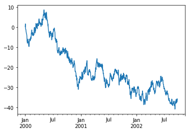
import matplotlib.pyplot as plt
ts=pd.Series(np.random.randn(1000),
              index=pd.date_range('1/1/2000', periods=1000))
ts=ts.cumsum()
ts.plot()
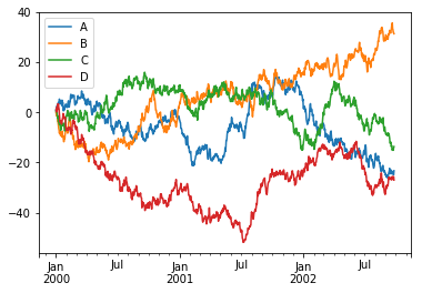
在DataFrame上,plot方法可以方便绘制所有带有便签的列
df=pd.DataFrame(np.random.randn(1000,4),index=ts.index,columns=['A','B','C','D'])
df=df.cumsum()
plt.figure()
df.plot()
plt.legend(loc='best')
获取数据
csv
写入csv文件
df.to_csv('foo.csv')
读csv文件
pd.read_csv('foo.csv')
HDF5
写入hdf5存储
df.to_hdf('foo.h5','df')
读取
pd.read_hdf('foo.h5','df')
excel
写入excel
df.to_excel('foo.xlsx',sheet_name='sheet1')
读取
pd.read_excel('foo.xlsx','sheet1',index_col=None,na_values=['NA'])
陷阱
如果你执行一个操作,可能会看到一个异常
if pd.Series([False, True, False]):
    print('True')
ValueError: The truth value of a Series is ambiguous. Use a.empty, a.bool(), a.item(), a.any() or a.all().